Relating Work and Pressure Mathematically:
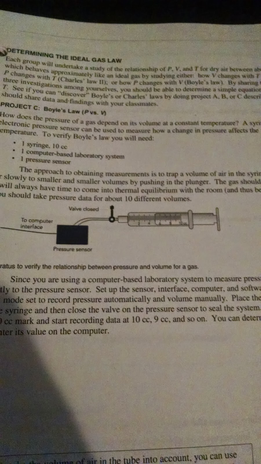
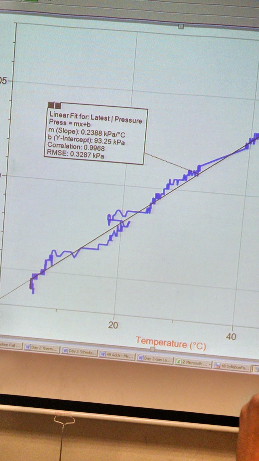
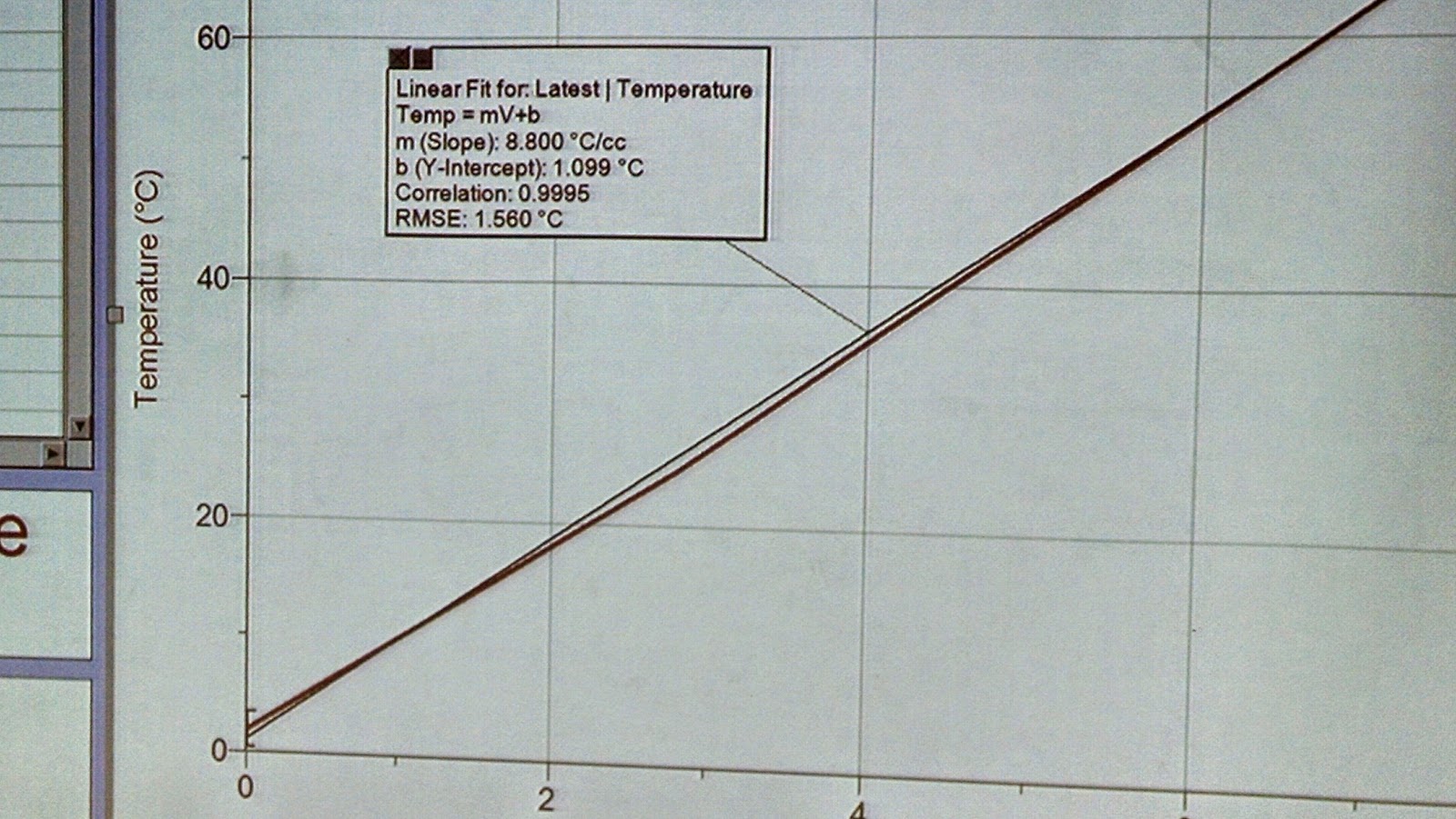
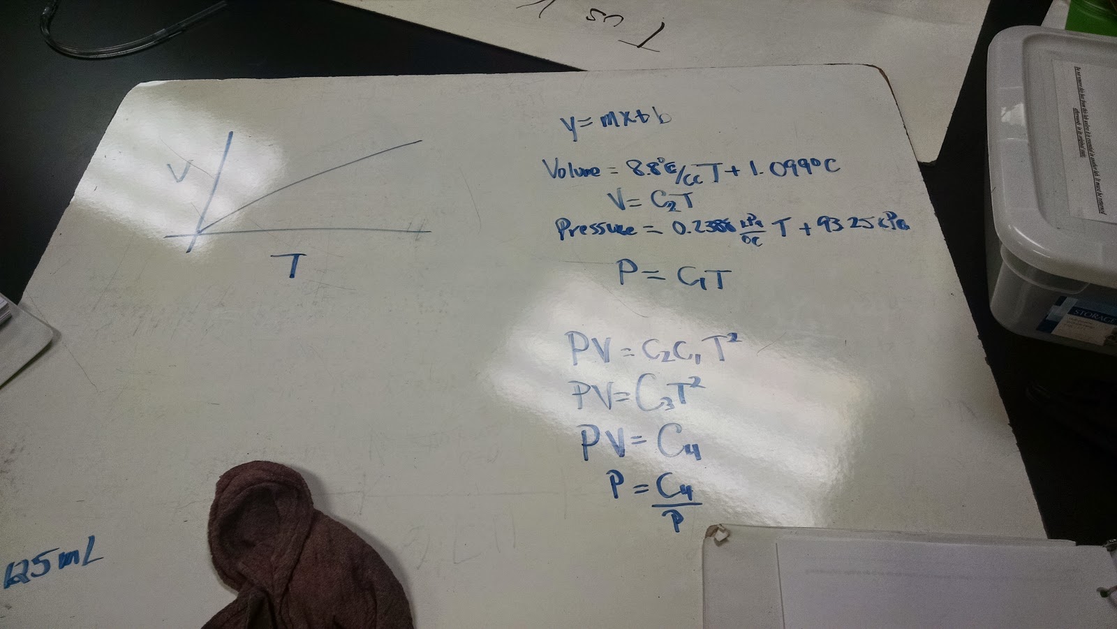
We first started this lab by bringing up the heated syringe lab activity we used to find the relationship between volume vs temperature. This time, however, we asked what occurs to the gas if we were to keep the plunger fixed. How would the gas react to keep itself at equilibrium
 |
| A revisit set-up from the last lab |
 |
| A demonstration of how to keep the plunger at bay. |
We find out that in order for the plunger to stay at a fixed distance, that work has to be applied onto the plunger by an external factor (in this case, Prof Mason's index finger) in order for the plunger to stay fixed. Of course, when the index finger is removed, so is the external work done to the plunger, and it is free to move up, as it should.
 |
| Giving this term of work a mathematical definition |
We moved straight along to give a definitive definition of work, which we find out to be the integral of Fdr, where F is the force, and dr is the differential of the distance moved.
To take the definition a bit further, we took the idea of Force, which is Pressure x Area, and substituted it for force. Realizing that Adr (which we made dx to give the term familiarity) is just dV (area being meters squared, and dx being meters), we then derive the term that work is equal to the integral of pressure by the change in volume
To take the definition a bit further, we took the idea of Force, which is Pressure x Area, and substituted it for force. Realizing that Adr (which we made dx to give the term familiarity) is just dV (area being meters squared, and dx being meters), we then derive the term that work is equal to the integral of pressure by the change in volume
 |
| Finding Work |
The first part gives us mass, ΔT, and pressure, and we are to find the work applied, in which case we first needed the final pressure, which was unknown as well.

The second part of the problem asked us to first find the Q (heat), and once we found Q, we then find the ΔU (internal energy) of the system.
Finding Q was just the process of Q=mcΔT
Finding ΔU used the idea of the First Law of Thermodynamics, since we have now both Q and W
Finding Q was just the process of Q=mcΔT
Finding ΔU used the idea of the First Law of Thermodynamics, since we have now both Q and W
2D Molecular Motion and Pressure:
We started this lab by using a 2D simulation of a diatomic atom at near absolute zero, and steadily increased the temperature to see what occurs.
 |
| Atoms in motion computer simluation |
We find out quickly that as the temperature reached to a certain point, the London Dispersion Force that was holding them apart broke, and the diatomic particle became two mono-atomic particles, bouncing faster and creating more work and pressure, the more that the temperature was increased in the system.
 |
| Larger amount of atoms in motion computer simulator |
We took that idea to the next level by adding more atoms to the system, ideally colliding in a perfectly elastic collision, thereb increasing the pressure, and once again increasing the work of the system, as the temperature was added in. Additionally, the path in which the atoms take became harder to notice, as more atoms were added to the system.
(Interestingly enough, the simulation crash after a while, unable to handle to handle it)
We took this idea, expanded it to a 3D situation, and tried to solve for various terms.
 |
| Finding our velocity component, and their Vtotal |
We were first asked to find the equations needed to calculate the x,y, and z components of velocity using X,Y, and Z and their time components.
Once we found these equations, we then needed to find the Vtotal in terms of the x,y, and z components.
While answering this question, we assumed that Vx=Vy=Vz, and was able to simplify the final results to be easier to work with.
Once we found these equations, we then needed to find the Vtotal in terms of the x,y, and z components.
While answering this question, we assumed that Vx=Vy=Vz, and was able to simplify the final results to be easier to work with.
 |
| Finding time |
We were then asked to find Δt in the x-direction, which is the amount of time the molecule to go from the left wall, bounce off the right wall, and head back to the left wall
Since we noticed that the movements of the ball is just Δt=2Δtx, we substituted that in to Δt
Since we noticed that the movements of the ball is just Δt=2Δtx, we substituted that in to Δt
 |
| Finding amount of force exerted |
We can then, using the idea of F=Δp/Δt (the true Newton's Second Law) and the equation we used to find time, to find the amount of force exerted on each collision
 |
| Expressing Fx |
Once we had an idea of the amount of force exerted, we can then substitute the expression we had to find the velocity of each component (the very first equation we derived) in order to find an expression just for Fx
We then took the idea of a cubical box with the length=width=height, making the volume V= X^3. By understanding the concept of pressure= force/area, we can then use it to express the pressure on the wall of this cubical box, caused by Fx and due to a single atom.
However, if we wanted the expression of Fx due to a N amount of terms Vtotal, we need to add in the idea that V=x^3 and understand the equation of vtot that we calculated early in the system ([vtot]^2= 3 vx^2] and can rewrite it to find pressure as function of vtot and V(pressure)
Additionally, understanding that mvtot^2 is just kinetic energy, we can again rewrite the equation as a function of Kinetic Energy
 |
| Expressing Pressure |
 |
| Two different expressions of Pressure (due to Fx and P) |
Additionally, understanding that mvtot^2 is just kinetic energy, we can again rewrite the equation as a function of Kinetic Energy
Gas Law and Kinetic Energy
Understanding the idea of the ideal gas law in terms of PV = NkbT, we also understand the following relationships
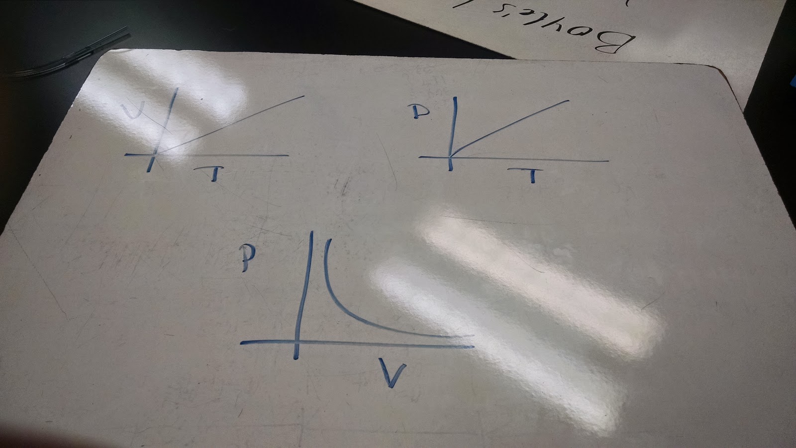
As the volume increases - the pressure decreases
As the number of particles increases - the pressure increases
Microscopic Definition of T
Understanding the idea of the ideal gas law in terms of PV = NkbT, we also understand the following relationships
As the volume increases - the pressure decreases
As the number of particles increases - the pressure increases
Microscopic Definition of T
 |
| Relationships between N,P, and V to kinetic energy (right side) Relating <Ekin> and T (left side) |
We can take the ideal gas law, and show that PV=2/3N<Ekin> (as shown on the left side).
Additionally, by sing the derived form of Ekin and T, we can then play around with the equation to obtain the vrms, or the root mean square velocity of molecules.
Isothermal Compression of Gas
We next learned about isothermal and adiabetic compression of gas
In this first picture, we show that Eint = 3/2NkbΔT
We then can understand that in an isothermal compression, temperature remains constant throughout. Using the ideal gas law, we can state that pV=nRT, and since nRT is a constant, we learn that pV= constant, and p1V1=p2V2
Additionally, since in an isothermal compression, there is no change in internal energy, that heat and work must them be equal to each other
Adiabetic Compression of Gas
 In an Adiabetic Compression, however, pressure is constant. With pressure being constant, we then find that the heat must then be zero, and that ΔE = -W. By reiterating that ΔE = 3/2NkbΔT and that work equals to -pΔV, we can then play with the equation, and with a little bit of integration, create the equations that expresses adiabetic compression of a gas.
Additionally, we must understand that the equation for an adiabetic equation shown here is only in cases of monotonic gases, and in diatomic gases require an extra two dimensions of freedom, thereby increasing from 3/2 to 5/2
The Fire Syringe - Fahrenheit 451:
In our last experiment, we were allow to spontaneously combust a piece of paper (or in our case cotton ball) using a fire syringe (which uses an adiabetic compression when done fast enough) and compare it to the "flash-point" of paper, which is 451°F
Before allowed to do the experiment, we needed to first calculate, using the Δh, the ΔV and the ΔT, the temperature that we should reach, and whether or not we should reach the flash-point
With our calculations, we calculated our temperature to be about 752K (error on my part of the °C) which is about 900°F, over double of how much we need to reach the flash-point
Although hard to see due to the video's sudden light issues, we do in fact create a spark with the cotton ball.
Additionally, to ensure that our experiment was a success (and to try to capture a better video) we attempted this experiment twice more, obtaining a spark (and a bad video) each time.
Conclusion:
Overall, we were able to successfully progress ourselves from the ideal gas law that we experimented from the last lab, into adiabetic and isothermal compression, through the usage of the Ideal Gas Law, and the First Law of Thermodynamics. We learned how to express the ideal gas law in the form of 3/2NkbT, which we then used to understand ΔE, helping understand the First Law of Thermodynamics, and ultimately leading to isothermal and adiabetic compressions (and causing cotton balls to spontaneously combust as well).
Additionally, by sing the derived form of Ekin and T, we can then play around with the equation to obtain the vrms, or the root mean square velocity of molecules.
Isothermal Compression of Gas
 |
| Equation of Isothermal compression |
In this first picture, we show that Eint = 3/2NkbΔT
We then can understand that in an isothermal compression, temperature remains constant throughout. Using the ideal gas law, we can state that pV=nRT, and since nRT is a constant, we learn that pV= constant, and p1V1=p2V2
Additionally, since in an isothermal compression, there is no change in internal energy, that heat and work must them be equal to each other
Adiabetic Compression of Gas
Additionally, we must understand that the equation for an adiabetic equation shown here is only in cases of monotonic gases, and in diatomic gases require an extra two dimensions of freedom, thereby increasing from 3/2 to 5/2
The Fire Syringe - Fahrenheit 451:
 |
| Our fire syringe and caliper needed for the experiment |
 |
| Our calculations and prediction for the combustion of the cotton ball |
With our calculations, we calculated our temperature to be about 752K (error on my part of the °C) which is about 900°F, over double of how much we need to reach the flash-point
 |
| Our video of the activity (Due to the sudden spark, my camera went wacko) |
Although hard to see due to the video's sudden light issues, we do in fact create a spark with the cotton ball.
Additionally, to ensure that our experiment was a success (and to try to capture a better video) we attempted this experiment twice more, obtaining a spark (and a bad video) each time.
Conclusion:
Overall, we were able to successfully progress ourselves from the ideal gas law that we experimented from the last lab, into adiabetic and isothermal compression, through the usage of the Ideal Gas Law, and the First Law of Thermodynamics. We learned how to express the ideal gas law in the form of 3/2NkbT, which we then used to understand ΔE, helping understand the First Law of Thermodynamics, and ultimately leading to isothermal and adiabetic compressions (and causing cotton balls to spontaneously combust as well).